
Volga Introduction — Open-Source Real-Time Data Processing Engine for AI/ML — Part 2
This is the second part of a 2-post series giving Volga’s high-level architecture overview and few technical details. For motivation and the problem’s background, see the first part.


TL;DR
Volga is an open-source real-time data processing/ML feature calculation engine providing a unified compute layer, data models and consistent API for different types of features: Online, Offline, On-Demand (see previous post) as well as a general purpose streaming engine.
It is built on top of Ray with a push+pull architecture and aims to remove dependency on complex multi-part computation layers in real-time ML systems (Spark+Flink/Chronon) and/or managed feature platforms (Tecton.ai, Fennel.ai, Chalk.ai).
Content:
Architecture Overview
API Overview - DataStream API and Entity API
Pipeline Example - The Push Part
On-Demand Compute Example - The Pull Part
Scalability
Deployment
Current State and Future Work
Architecture overview

Volga’s main goal is to provide a consistent unified computation layer for all feature types described in the previous post (Online, Offline and On-Demand). To achieve this, it is built on top of Ray’s Distributed Runtime and uses Ray Actors as main execution units. Let’s look at the moving parts of the system:
Client — The entry point of any job/request. Users define online and offline feature calculation pipelines using declarative syntax of Operators:
transform,filter,join,groupby/aggregate,drop(see examples below). Client is responsible for validating user’s online/offline pipeline definitions and compiling them intoExecutionGraph, On-Demand feature definitions intoOnDemandDAG(Directed Acyclic Graph).Streaming Engine Workers — Ray Actors executing streaming operators based on
ExecutionGraphfrom client. Volga is built using Kappa architecture so stream workers perform calculation for both online (unbounded streams) and offline (bounded streams) features. Calculation is performed on Write Path (asynchronously to user request). Message exchange between workers is done via ZeroMQ.On-Demand Compute Workers — Ray Actors executing
OnDemandDAGof on-demand tasks. Performed on Read Path (synchronously to user request), result is immediately returned to a user. On-demand workers pull pipeline’s results (based on user-defined DAG of features) from the storage at request time and perform needed computations based on parameters specified in user’s request (keys, ranges, custom args). These features can also be simulated in offline setting (provided users timestamps/request data).Data/Storage Connectors — Volga comes with a set of configurable data connectors, two main base classes are
PipelineDataConnectorandOnDemandDataConnectoreach of which incapsulates logic for their respective execution flows (pipelines and on-demand respectfully, more about this in a separate post). In the diagram above, we have outlined two logically separet types of storage that are commonly used in real-time ML systems: ColdStorage for offline setting and long term/high volume data (e.g. MySQL, data lakes, etc.) and HotStorage for real-time high-throughput/low-latency data access (e.g. Redis, Cassandra, RocksDB).By default, Volga comes with a built-in
InMemoryActorStoragewhich is suitable for both pipeline and on-demand storage and can be used for local development/prototyping.
The graph above demonstrates a high level execution/data flow for each feature type -Online (red), Offline (blue), On-Demand (green).
API Overview - Entity API and DataStream API
Volga provides two sets of APIs to build and run data pipelines: high-level Entity API to build environment-agnostic computation DAGs (commonly used in real-time AI/ML feature pipelines) and low-level Flink-like DataStream API for general streaming/batch pipelines.
In a nutshell, Entity API is built on top of DataStream API (for streaming/batch features calculated on streaming engine) and also includes interface for On-Demand Compute Layer (for features calculated at request time) and consistent data models/abstractions to stitch both systems together.
Entity API distinguishes between two types of features: @pipeline (online/streaming + offline/batch which are executed on streaming engine) and @on_demand (request time execution on On-Demand Compute Layer), both types operate on @entity annotated data models.
In general, if you want to do feature engineering in ML, Entity API is your best bet. If you have some other streaming use case and want to use Volga solely as a streaming engine or just need more flexibility, use DataStream API.

Sample Pipelines - The Push Part
Let’s start with an example of how to use Entity API. Assume we want to build pipelines where we have users (one source/data store) making purchases (another source) and we need some joined aggregate statistics (e.g. number of purchases on sale in the last hour) which we want to derive from both historical data and access at real-time.
All of the streaming/batch feature calculation pipelines rely on Volga’s Streaming Engine - The Push Part and are annotated with @pipeline decorator.
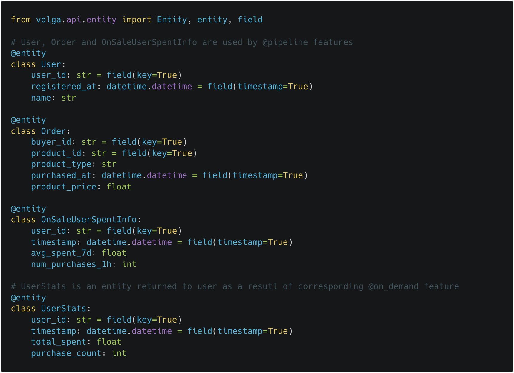
First, use
@entityto decorate data models. Notekeyandtimestamp: keys are used to group/join/lookup features, timestamps are used for point-in-time correctness, range queries and lookups by on-demand features. Entities should also have logically matching schemas - this is enforced at compile-time which is extremely useful for data consistency.
Define pipeline features (streaming/batch) using
@sourceand@pipelinedecorators. We explicilty specify dependant features independencieswhich our engine automatically maps to function arguments at job graph compile time. Note that pipelines can only depend on other pipelines

See how we declaratively define our pipeline transformations using Pandas-like syntax - using Kappa architecture, our streaming engine will make sure that when executing this pipeline we will get consistent results for both online and offline setting.
Note that we can also pass parameters to our pipeline definitions which can help us build custom streaming job topologies depending on different use cases, e.g. using different sources for online and offline execution.
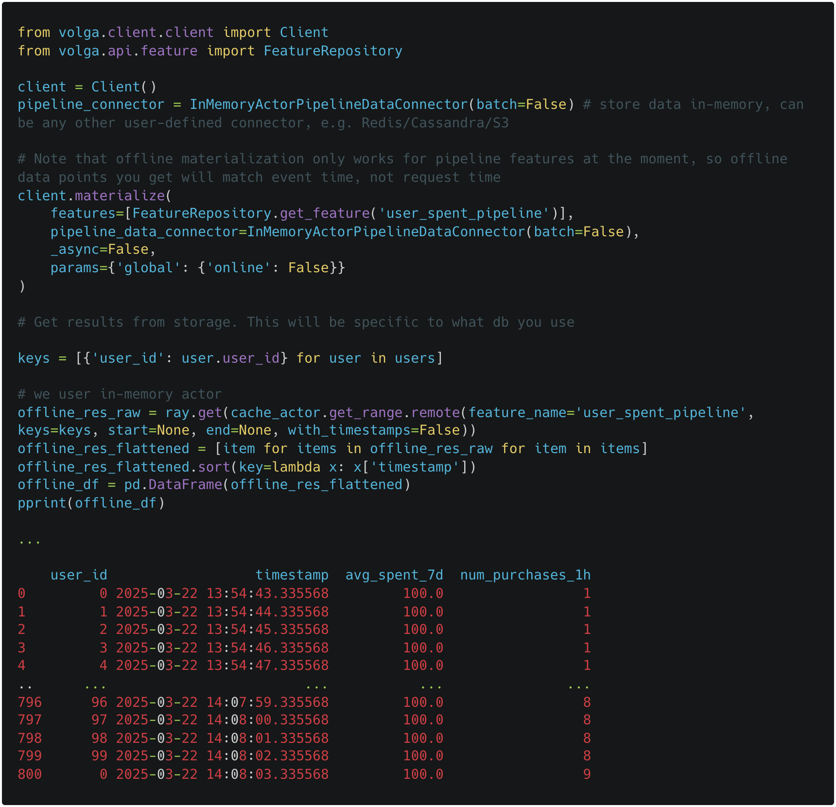
Now let’s run batch (offline) materialization which will execute pipeline and store data using configured PipelineDataConnector (e.g. to generate historical features for model training).
Now let’s see how we can combine On-Demand Compute and online materialization to get features in real-time.
On-Demand Compute - The Pull Part
On-Demand Compute layer (or the Pull Part of the system) allows performing stateless transformations (or graphs of transformations) at user request time, both in online and offline setting. This can be helpful in cases when transformation is too performance-heavy for streaming or when input data is available only at inference request time (e.g. GPS coordinates, meta-model outputs, etc.).
For our case, On-Demand Layer will be needed to serve online pipeline output and enrich it before returning to the user.
Define on-demand features using
@on_demand- this will be executed at request time. Unlike@pipeline,@on_demandcan depend on both pipelines and on-demands. If we just want to serve pipeline results, we can skip this.

Launch asynchronous streaming (online) materialization job, it’s outputs will be pulled by On-Demand workers based on the logic defined in OnDemandConnector (defined in the next step)

In a separate thread/process/node or whatever service that needs to access the features, initialize OnDemandClient and use it to request feature results in real-time. Note that we also launch On-Demand Workers here via coordinator - this step can be done from any other place.

Scalability
For the streaming engine, Operators have a notion of parallelism (similar to Flink’s parallelism) — As an example, consider a simple Order.transform(…) pipeline from previous example. Compiling this pipeline into a JobGraph will create the following structure:
SourceOperator → MapOperator → SinkOperator
By default, when JobGraph is translated into ExecutionGraph, if all operators have parallelism of 1, ExecutionGraph will have the same 3 node structure. Setting parallelism to 10 will result in an ExecutionGraph consisting of 10 copies of the above 3 node structure, creating 10 similar pipelines (note that it is up to a user to implement partition/storage logic for sources and sinks based on operator index in a given graph). This works for both offline (bounded streams) and online (unbounded streams) features.
Volga also allows setting resource requirements (such as CPU shares and heap memory) via ResourceConfig. This can be done globally, per-job or per-operator.
For On-Demand Layer, we can specify num_servers_per_node - all of the requests will be round-robined between them.
Running locally and deploying to remote clusters
Volga runs wherever Ray runs, meaning you can launch it locally, on a Kubernetes cluster with KubeRay, on bare AWS EC2 instances or on managed Anyscale.
For local env, just run ray start —head and run your pipeline. See Volga Ops repo for more examples.
Current state and future work
Volga is currently in active development but requires a number of features to get to a prod-ready release, check out the roadmap here:
The high level architecture has been validated and tested, the main moving parts of streaming engine are in place and have been tested (including scalability and networking), on-demand layer is done, user facing API and data models are done. The ongoing work mainly involves fault tolerance, data connectors implementations and load testing/scalability testing.
Thank you for reading and please share, star the project on Github, join us on Slack and most importantly, leave your feedback as it is the main motivation behind this effort.