

TL;DR
Volga is an open-source real-time data processing engine for AI/ML workloads. It focuses on problems common in real-time ML systems: consistent online/offline feature computation, point-in-time correct aggregations, long sliding windows, and ML-oriented functions such as top and categorical aggregations.
This post walks through the Rust rewrite of Volga, built on Apache DataFusion, Apache Arrow, and SlateDB. We also compare its architecture with ML-oriented systems like Chronon and OpenMLDB, and general streaming engines such as Apache Flink, Apache Spark, and Arroyo.
Content:
Background
Rewriting Volga in Rust
High-level Architecture
Streaming + Batch execution modes: Dataflow and Incremental Compute
Request execution mode: Read–Write Compute Separation and Queryable State
Window Aggregations: Tiling and Custom Aggs (
top,_cate,_cate_where)Remote State Storage: Compute-Storage Separation
Comparison with existing systems
Current state and future work
Background
Modern real-time ML systems (e.g. recommendation systems, fraud detection, personalized search, RAG pipelines) rely on features computed from event streams such as user activity, transactions, or logs. These features are typically defined as aggregations over recent events — for example “number of purchases in the last hour” or “average transaction value over the last 7 days”. In practice this means continuous sliding window aggregations, which are the core building block of many feature pipelines.
Such systems introduce several challenges: maintaining consistent feature definitions and computation semantics between online and offline pipelines, supporting point-in-time correct aggregations for training and inference, and efficiently computing long windows at high ingest rates.
General-purpose engines like Apache Flink or Apache Spark can implement these pipelines, but require additional infrastructure (intermediate storage, serving layers, feature definition DSLs) and non-trivial performance tuning. As a result, systems like Chronon and OpenMLDB appeared to address parts of this problem in open source, while platforms like Tecton (recently acquired by Databricks) provide a managed solution - you can find more details in previous blog post.
Volga is an open-source, self-hostable and standalone engine focused on efficient continuous window aggregations expressed in SQL, with unified streaming, batch, and request-time execution, optimized for AI/ML workloads. The project originally started as a Python-based system on Ray; the current Rust implementation revisits the architecture, combining ideas from Chronon and OpenMLDB while improving performance, simplicity and overall .
Rewriting Volga in Rust
The first iteration of Volga was implemented mostly in Python, with some low-level performance-critical components, such as networking, already written in Rust (see previous blog post on networking stack). It used native Python operators running on top of Ray Actors as the execution and orchestration layer. This setup enabled rapid prototyping and provided acceptable performance and scalability for streaming workloads (see benchmarking post), but had several drawbacks, the main one being performance, especially when used as a batch processor.
The current version of Volga is implemented in Rust, providing better performance, memory control, and concurrency via Tokio async runtime.
DataFusion
Apache DataFusion is a Rust-native query framework that provides SQL parsing, query planning, and a vectorized execution engine for building data processing systems.
This allows Volga to move from custom Python DataFrame API to pure SQL (extensible to DataFusion’s own DataFrame API) by using DataFusion’s SQL Query Planner to construct a consistent dataflow graph used across all execution modes. Using SQL provides a powerful and familiar way to describe both general data pipelines as well as feature transformations in ML workloads. Volga also uses DataFusion for schema handling, expression evaluation, and utilities such as hashing, window expressions, and aggregation abstractions, while extending it with custom window functions and accumulators.
Arrow
Apache Arrow provides the in-memory data representation used across the system. Volga processes all data as Arrow RecordBatches, and Apache DataFusion uses Arrow as its underlying execution format.
Processing data in columnar batches allows operators to work efficiently while maintaining a streaming execution model. Many operators rely on Arrow compute kernels — optimized vectorized functions operating on columnar arrays — which improves performance by reducing per-record overhead.
SlateDB
One of the key goals of Volga is to provide compute and storage separation - we want to keep operator’s state outside the execution workers, which allows for independent compute and storage scaling as well as more efficient data movement, significantly reducing overall resource usage.
SlateDB is used as the state storage layer. It is an embedded LSM-tree key–value store designed to run on top of cloud object storage (S3), making it well suited for streaming workloads where state is continuously updated.
Being embedded, SlateDB runs directly inside the Volga worker process rather than as a separate service, avoiding network roundtrips on the state access path. Its LSM-tree design provides efficient writes and compaction, which fits the update-heavy nature of streaming state (windows, joins, aggregations).
High-level architecture overview
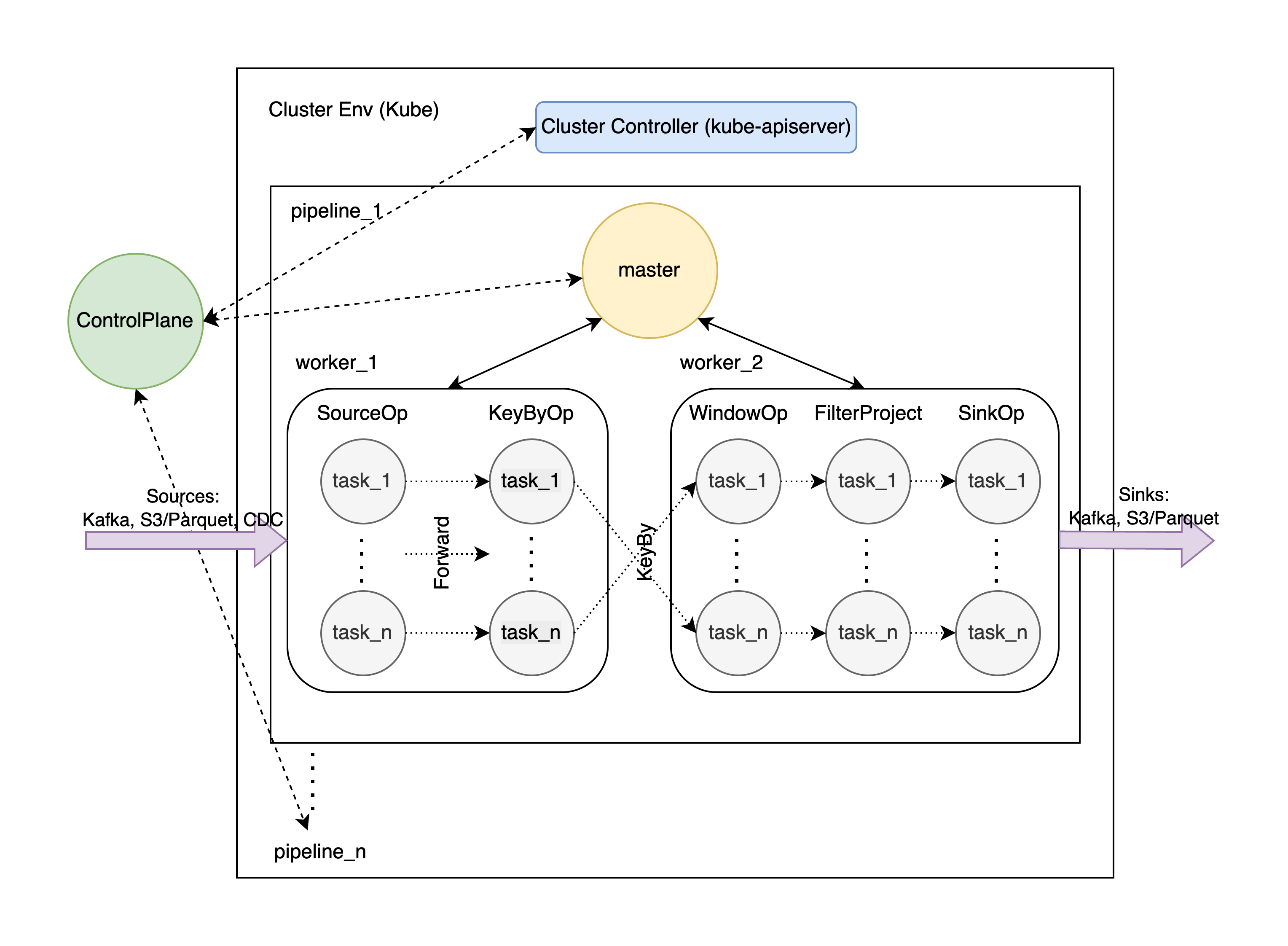
Volga is a Distributed Dataflow system consisting of a Control Plane and a runtime composed of Masters, Workers, and Operators executed in parallel Tasks.
Control plane
The control plane exposes APIs to create, update, and delete pipelines (jobs), handling interaction with the cluster runtime environment (such as Kubernetes or Ray) and managing deployment and resource allocation for pipelines. Pipeline metadata and lifecycle state are stored in a SQL-compatible backend (e.g. PostgreSQL), allowing pipelines to persist across restarts.
Master and Workers
Each pipeline runs as a Master–Workers cluster.
The Master manages the pipeline lifecycle: compiling the execution graph, assigning tasks to workers, collecting telemetry, and coordinating checkpointing.
The Workers execute the dataflow graph. They run operators, maintain state when required, and exchange data using gRPC streaming for remote communication and Tokio channels for local communication.
Operators, Tasks, Parallelism and Partitioning
A pipeline is compiled into a dataflow graph of operators, each representing a transformation on one or more streams (for example map/filter, joins, window aggregations, or sources and sinks). Operators can be stateless or stateful, persisting state in the storage layer.
A task is the physical execution unit of an operator. Each task runs in its own Tokio runtime (providing resource isolation) and executes an async actor implemented with Kameo together with the I/O Tokio tasks associated with that operator.
Operators can run with configurable parallelism, meaning multiple tasks execute the same operator concurrently. Data is distributed between tasks using partitioning strategies:
Forward– one-to-one transfer when upstream and downstream parallelism matchHash– ensures records with the same key go to the same task (used for windows and joins)RoundRobin– distributes records evenly across tasks
At runtime, the control plane provisions the pipeline runtime, the Master compiles the query into an execution graph and assigns tasks to workers, and workers begin processing data while the Master coordinates telemetry and checkpointing.
Volga supports 3 pipeline execution modes - Streaming, Batch and Request
Streaming + Batch execution
As a general-purpose data processing engine, Volga supports both Streaming and Batch execution modes. In AI/ML pipelines, streaming mode is used to compute and continuously update features, acting as a backbone for Request Mode (described below), while batch execution can be used to compute training datasets.
Volga uses Dataflow model, where computations are represented as a directed graph of operators processing data. Operators maintain state and exchange records through the graph while watermarks propagate logical event-time through the pipeline. This allows the same execution engine to support both continuous streaming computation and bounded batch processing.
Streaming execution: watermarks, out-of-orderness, and stateful processing
In streaming mode, operators process events according to their event-time. A key challenge is logical disorder: events may arrive out-of-order relative to their event-time. This may originate from upstream sources or from the system itself due to network delays or data shuffling across workers.
To handle this, Volga uses watermarks, which represent the engine’s estimate of event-time progress. When a watermark reaches an operator, it indicates that no earlier events are expected, allowing the operator to safely emit results or advance window computations.
Volga generates watermarks using a bounded out-of-orderness assumption, similar to the approach used in Apache Flink. Events are allowed to arrive within a configurable delay relative to their event-time; anything outside this bound is considered late and is currently dropped.
Operators such as windows and joins are stateful, meaning they retain intermediate data to produce correct results. For example, window aggregations keep records belonging to the current window, while joins store records from both sides until matching events arrive.
Fault tolerance, checkpointing, and exactly-once processing
Volga provides fault tolerance through distributed checkpointing based on the Chandy–Lamport snapshot algorithm.
The master periodically instructs sources to inject checkpoint barriers into the dataflow. As these propagate through the pipeline, stateful operators snapshot their state, producing a consistent checkpoint of the entire graph. If a worker fails, the pipeline is restarted from the latest checkpoint.
If sources support exact replayability (for example using offsets in Apache Kafka), Volga guarantees exactly-once processing. Even if events are replayed during recovery, the resulting state and outputs are identical to a failure-free execution.
Incremental Computation and Update Handling
The current computation model in Volga is built around append-only data — a stream of events where records are only added. This works well for many scenarios (logs, transactions, user activity), where data naturally accumulates over time. However, when working with Change Data Capture (CDC) sources, this assumption breaks: the source starts emitting changes (updates and deletes), aggregates lose their monotonicity, previously computed results may need to be recomputed, and watermarks no longer guarantee that “the past is complete.”
Changelog Streams and Retract (Flink-style approach)
One option is to extend the current dataflow model to support changelog streams, similar to Apache Flink. In this model, records exchanged between operators are not just events but changes with a type (INSERT, UPDATE, DELETE, or UPDATE_BEFORE / UPDATE_AFTER pairs).
This requires operators to support incremental state updates: they must be able to apply changes and, when necessary, retract previously applied values. As a result, outputs also become changelog streams rather than append-only results. This approach preserves the existing dataflow + watermark architecture, but increases complexity: operators need to maintain additional state, and some aggregations (e.g. top-k or min/max) require non-trivial retract logic.
Differential Dataflow
An alternative approach is to adopt a Differential Dataflow model: data is represented as a stream of changes (diffs), where each record carries a weight (e.g. +1 or -1), and updates are expressed as a combination of removing the old value and adding the new one.
Computation is defined through algebra over these weights: changes can be accumulated and canceled out, and in operations like joins, weights are combined (e.g. via multiplication). This allows changes to propagate naturally through the dataflow graph without requiring explicit retract logic in each operator.
Instead of event-time and watermarks, a more general notion of time is used: each record carries a logical timestamp, and progress is tracked via frontiers — sets of timestamps for which updates may still arrive. Unlike linear watermarks, this allows the system to operate over partially ordered time.
As a result, system state is defined as the accumulation of all changes up to a given point in time, and update/delete handling becomes a natural part of the model. This approach is more expressive, but also requires a significant architecture redesign.
Batch execution
In batch mode, the same dataflow graph is executed over a bounded dataset. The pipeline is evaluated as a sequence of stages, each updating the state of a single operator using all data produced by the previous stage. For example:
sources (a+b) → join → window → sink
execution stages are:
read all source data and build the join state
emit join results and update the window state
emit window results to the sink
Each stage first consumes all input data and then emits an end-of-input watermark (MAX_WATERMARK), triggering the operator to finalize its state and produce all remaining outputs.
Using the same operators for both streaming and batch ensures consistent semantics across execution modes. Batch execution support is currently a work in progress.
Data Shuffle
Data shuffle is the redistribution of data between tasks across workers (typically by key), ensuring correct data locality for operations such as aggregations and joins.
Streaming: data shuffle is currently implemented via shared gRPC streaming channels between workers (worker-to-worker), similar to pipelined shuffle in Apache Flink. The main issue is that multiple downstream tasks may share a single channel, and a slow consumer can introduce backpressure for all (head-of-line blocking). Possible solutions include adding credit-based flow control (as in Flink) or switching to per-task gRPC connections (task-to-task) to isolate consumers.
Batch: for batch workloads, a dedicated shuffle service with compute–storage separation is more appropriate. One option is S3-based (diskless) shuffle, where intermediate data is materialized in object storage and read by downstream tasks. Similar approaches are used in remote shuffle in Apache Spark (e.g. Apache Uniffle and Apache Celeborn), and are also being explored in the Apache Flink ecosystem.
Request-mode execution: Read–Write Compute Separation and Queryable State
Request mode allows Volga to serve query results directly to external systems by asynchronously reading the continuously updated state of streaming operators and performing the final aggregation at request time (e.g. serving features for model inference).
The design follows the write-time and read-time compute separation: the streaming pipeline continuously updates intermediate state (write path), while incoming requests read this state and compute the final result (read path). This idea is discussed in more detail in the Why AI Workloads Need Read and Write Computation blog post by zipline.ai (managed Chronon).
A common implementation is to run a streaming pipeline that materializes intermediate state (for example fixed-size pre-aggregated tiles) into an external hot storage (e.g Redis or MongoDB). A separate stateless serving layer then handles incoming requests by reading this state and performing the final aggregation. Systems like Chronon (built on Apache Flink or Apache Spark with external Key-Value storage) and earlier versions of Volga (separate streaming, cache, and serving workers - more here and here) follow this pattern.
Volga takes this idea one step further by embedding request-time processing directly inside the dataflow graph and querying streaming state directly. Incoming requests are treated as an additional input stream and processed by a dedicated request operator, which reads the state of adjacent streaming operators and performs the final aggregation. Streaming updates and requests are handled asynchronously, preserving read–write separation while avoiding materialization in external serving layers and reducing request latency by querying state directly.
Consider the following query:
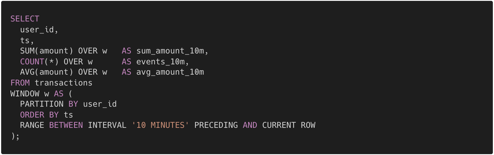
In streaming or batch execution mode, the planner produces the following graph:
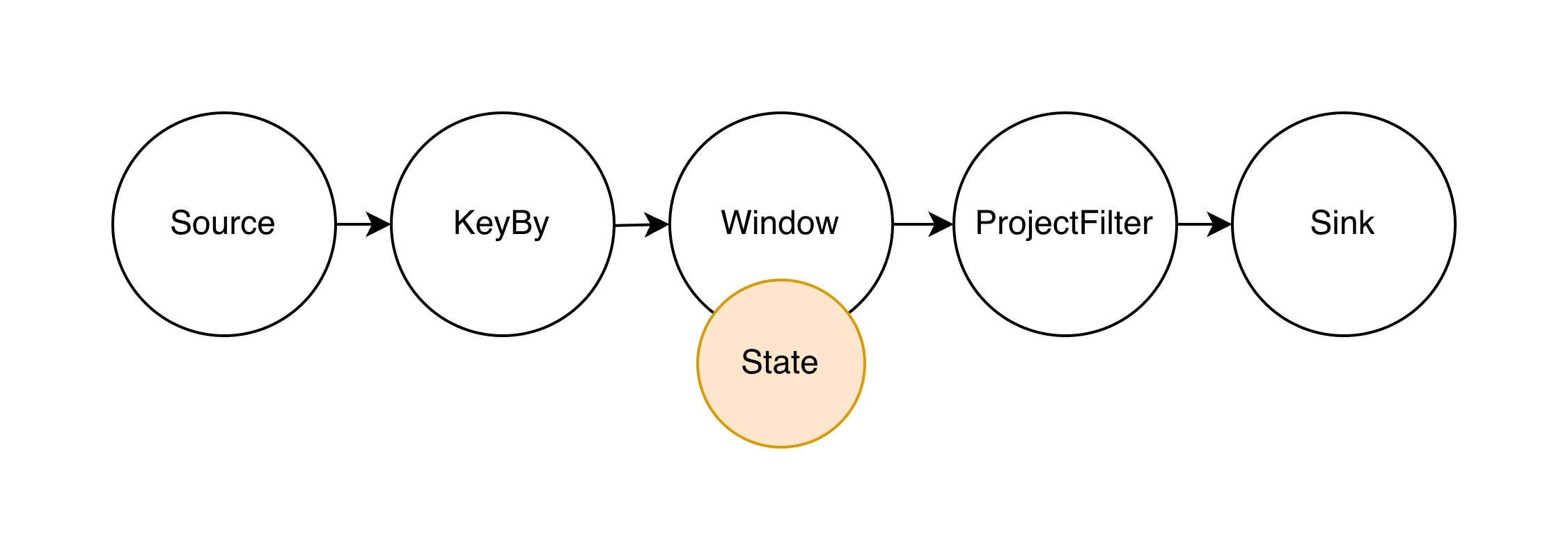
In request mode, the graph is modified with several additional components:
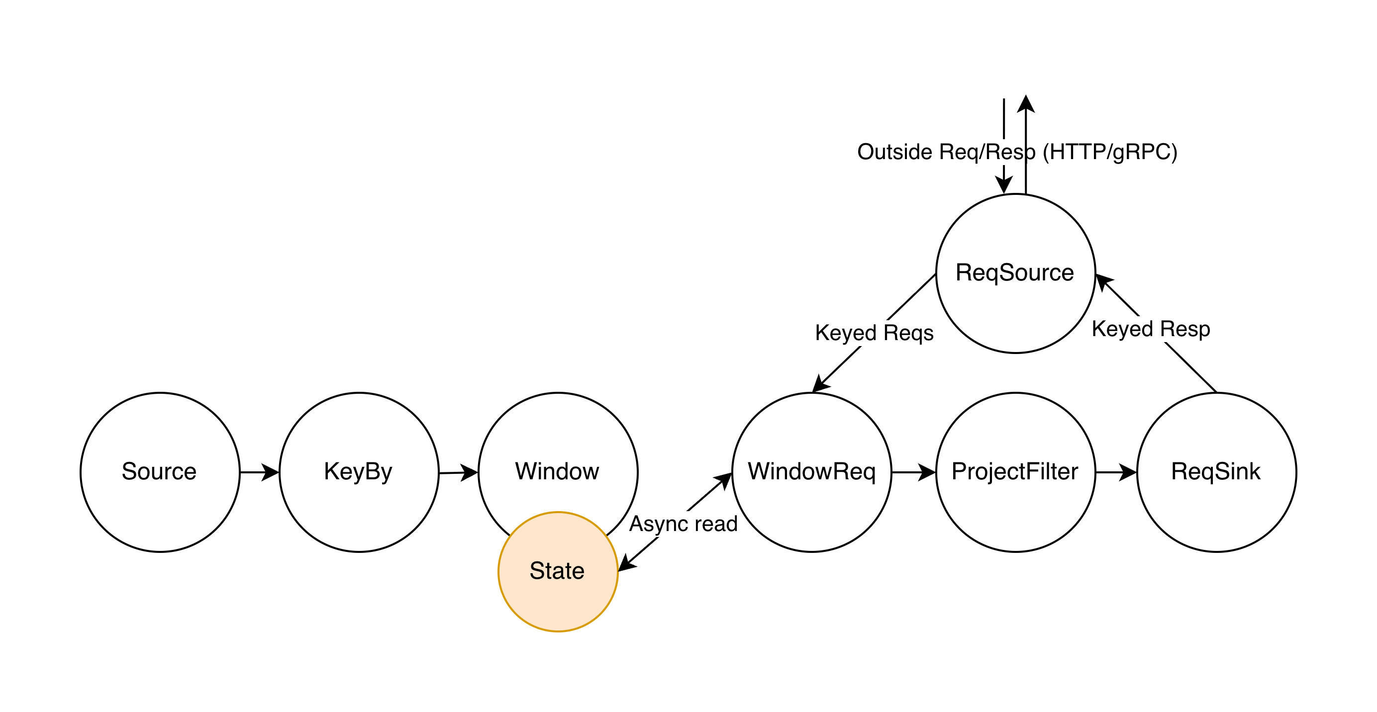
Three operators participate in request execution:
RequestSource– entry point for external requests. It exposes a service interface (currently implemented using Axum), queues requests, and waits for replies.WindowRequestOperator– processes requests by reading theWindowOperatorstate using the request key and computing the aggregation using the same logic as in streaming or batch mode. In request mode theWindowOperatoronly maintains state and does not emit results, which moves actual aggregation to read path.RequestSink– forwards the result back to RequestSource, completing the request–reply cycle.
This design reuses the same state and aggregation logic across streaming, batch, and request execution while keeping the serving path fully integrated into the engine.
An open question in this design is how to ensure high availability. In particular, what happens if a stateful operator fails? How can the system continue serving (possibly slightly stale) results while the streaming pipeline is being restored from a checkpoint and replaying the latest data from the source?
Window Aggregations
Window aggregations in Volga are executed by a dedicated operator that maintains per-key window state. The input stream is keyed using hash-based partitioning, and each partition is processed independently while the window frame continuously slides as new records arrive.
As rows enter the window, the operator updates aggregation accumulators. When the frame advances and rows fall out of the window, their contribution is removed if the aggregation supports retraction. Volga therefore distinguishes between retractable aggregations (e.g. avg, count, sum), which support insert and retract updates and only store their current state, and plain aggregations (e.g. min, max), which cannot retract and therefore keep the rows currently inside the window so the aggregate can be recomputed when needed.
Result emission is driven by watermarks, which track event-time progress and allow the engine to handle out-of-order data. As the watermark advances, the operator emits updated window results once the corresponding portion of the stream is considered complete.
Custom Window Aggregations
Inspired by OpenMLDB, along with general aggregation functions (min, max, avg, sum, count), Volga includes several SQL-native window functions designed for patterns commonly used in ML feature engineering. These allow many feature extraction tasks to be expressed directly in SQL instead of requiring separate preprocessing pipelines.
Internally these functions are implemented on top of Apache DataFusion’s User Defined Window Function (UDWF) interface. Each function maintains it’s state using a window Accumulator, which is incrementally updated as rows enter and leave the window frame. This allows the custom logic to integrate naturally with DataFusion’s execution model while preserving the performance benefits of incremental window evaluation.
Top aggregations
A common feature engineering pattern is identifying dominant or frequent values within a sliding window. Volga provides several built-in functions for this:
top(col, k)– returns the topkvalues in the window, ordered by valuetopn_frequency(col, k)– returns thekmost frequent values together with their frequenciestop1_ratio(col)– returns the dominance ratio of the most frequent value in the window
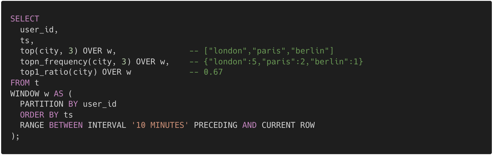
The implementation maintains compact frequency state inside the accumulator. For topn_frequency this consists of a frequency map combined with a small heap used to extract the top-k entries. top1_ratio tracks the maximum frequency together with the total number of elements in the window to compute the dominance ratio. Since the accumulator is updated incrementally when rows enter or leave the frame, the system avoids recomputing statistics for the entire window.
A similar computation in Apache Flink SQL typically requires a multi-stage query involving windowed aggregations followed by ranking functions such as ROW_NUMBER() and filtering the top entries. Volga exposes this pattern as a single window aggregation, making common feature engineering queries significantly simpler to express.
Categorical aggregations
Another common pattern in ML workloads is computing aggregates for specific categories within a window. Volga provides categorical variants of standard aggregations such as sum_cate, count_cate, avg_cate, min_cate and max_cate, together with conditional variants using _where and _cate_where.
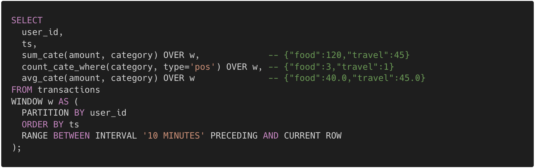
The implementation relies on Apache Arrow kernels for vectorized filtering and grouping, while the aggregation state itself is maintained inside a DataFusion accumulator. Internally the accumulator stores partial aggregates in a hash map keyed by the category value and updates the relevant entries as rows move through the window. This keeps the computation incremental while leveraging Arrow’s columnar execution model.
These extensions allow many ML-oriented feature engineering patterns to be expressed declaratively in SQL while remaining fully integrated with the Volga execution engine.
Long window aggregations and Tiling
One of the key requirements for AI/ML workloads is support for long time windows, often spanning months or even years. Combined with continuously sliding windows and high ingest or query rates, such workloads can become very compute-intensive on both the read and write paths. Traditional streaming engines such as Apache Flink and Apache Spark are generally not optimized for this pattern.
Systems like Tecton and Chronon address this using Tiling. During ingestion, the write path continuously materializes pre-aggregated values for fixed time intervals (tiles). At query or request time, the read path combines the relevant tiles to compute the final window result. This separates the heavy aggregation work from the ingestion pipeline and avoids scanning large volumes of raw events when computing long windows.
Volga implements this idea natively inside the window operator. Tiles are maintained as part of the window state and updated during stream processing. Both streaming and request-time queries reuse these tiles to compute final results, allowing Volga to support very long windows efficiently without relying on external intermediate storage.
Remote State Storage
Designing a storage layer for operator state requires supporting several constraints so the system works efficiently across streaming, batch, and request execution modes.
Key requirements
Compute–storage separation – State is stored remotely so compute and storage can scale independently and state does not need to move during checkpoint/restore. Traditional engines like Apache Flink or Apache Spark Streaming often colocate state with workers, which can lead to inefficient resource usage for larger states
Different read/write patterns
Batch mode – large writes once, then read all state for a key.
Streaming mode – frequent small writes and sequential reads.
Request mode – reads and writes happen asynchronously from different operators.
Time-aware data access – Data usually arrives mostly ordered by event time with occasional disorder. Reads must always produce a correct time-ordered view for a given window.
Partial state loading – Window state may contain raw events, indices, and tiles. Large windows should load only the required data (e.g. tiles plus minimal raw events).
Resource isolation – Workers may run many operator tasks. Local buffers and caches must enforce limits and share resources fairly.
Storage Layout
Incoming events first enter an in-memory WriteBuffer, which batches updates before asynchronously persisting them to remote storage. The buffer size can be tuned per execution mode or disabled entirely in batch mode.
For efficient time-based access, incoming batches are sorted by event time and split into fixed time buckets. Each key maintains a WindowState structure containing a BucketIndex mapping buckets to batch identifiers stored in the KV store.
WindowState also stores tiles — pre-aggregated values for fixed time intervals used to efficiently compute long windows.
On reads, Volga loads the WindowState, uses the BucketIndex and tiles to locate batches needed for a given time range, and loads only those batches. Since batches are already sorted, producing a time-ordered view simply requires merging them (cheap). A background maintenance task can periodically merge batches within buckets to avoid fragmentation.
A MemoryGovernor tracks memory usage of buffers and caches per operator task, triggering backpressure or flushing when limits are reached.
Persistent Storage
Persistent storage is implemented using SlateDB - an embedded LSM-tree KV store that uses object storage (e.g. S3) as its durable layer and integrates with Foyer for local memory and disk caching. This provides high write throughput and low-latency reads.
Because persistence is delegated to object storage, durability and replication are handled by S3, allowing Volga to avoid implementing its own replication layer and keeping the system simpler.
SlateDB also operates on versioned data, which makes checkpointing inexpensive: instead of copying state, Volga can snapshot a storage version. This makes checkpoint restore very cheap, unlike in Apache Flink where large state transfers over the network are often required.
The result is an LSM-tree–backed, merge-on-read, time-bucketed storage layer on top of object storage, providing scalable remote state with high throughput and low-latency access.
Open Questions
The storage layer is a work in progress and several design questions remain:
Can the two-step read (load state → load batches) be simplified using LSM-Tree range scans?
How should concurrency control work in request mode when reads overlap with window eviction?
How should pipeline rescaling redistribute state when each worker owns its own SlateDB instance (considering SlateDB is a single writer system)?
Where should compaction run — per worker, per pipeline, or centrally?
Is an LSM-tree optimal for batch workloads, where data is written once and read all at once?
Comparison with Existing Systems
The systems below are more mature and production-ready, while Volga is still a work in progress. The comparison therefore focuses on core architectural design choices, not feature completeness.
vs Flink / Arroyo
All three systems are Dataflow-based streaming engines with event-time processing and watermarks.
Flink and Arroyo are general-purpose engines with broad SQL functionality. Volga instead focuses on continuous window aggregations, which dominate real-time ML feature pipelines (no general GroupBys, exepects time to be semantically present) and also includes ML-oriented aggregations such as top and categorical aggregations (_cate, _where), which are harder to express in general Flink-like SQL.
Another key difference is state architecture. Volga is designed around remote state storage, enabling compute–storage separation.
Volga also provides a native request execution mode, where external requests query operator state directly inside the dataflow graph. In ML feature serving architectures built on Flink or Arroyo, this serving layer typically needs to be implemented separately.
Architecturally, Volga is closest to Arroyo: both are written in Rust and use Apache DataFusion for SQL planning. However, Arroyo relies on DataFusion’s built-in window execution (WindowAggExec), while Volga implements custom window operators optimized for remote state instead of DataFusion’s in-memory batch state model.
vs Chronon
Both systems target real-time ML feature computation and follow the write/read compute separation pattern: a streaming pipeline maintains intermediate state while requests read that state to compute final results.
The main difference is system composition: Chronon combines multiple systems such as Flink, Spark with external Key-Value storage (e.g. MongoDB or Redis) and a custom serving layer. Volga instead aims to provide a single standalone runtime written in Rust, integrating streaming execution, storage, and request processing. Since Chronon depends on Flink-based streaming, it also inherits some state management limitations typical for those systems.
Another key difference is that Volga uses SQL for feature definitions, while Chronon relies on a custom DSL.
vs OpenMLDB
OpenMLDB is a real-time database optimized for ML feature queries, where most computation happens at read time. Volga instead separates work to write path (during ingestion using streaming pipelines) and read path (request serving).
Key architectural differences:
Execution model
Volga: streaming ingestion (via native streaming sources) + asynchronous request reads
OpenMLDB: bulk ingest (needs outside actor to perform writes), query-time computation
Storage
Volga: remote state backed by object storage (e.g. S3)
OpenMLDB: local to compute, in-memory + disk
In practice both systems can achieve similar read/request latency, but they make different trade-offs.
Because Volga relies on watermark-based streaming execution, feature freshness depends on watermark configuration. Tight watermarks improve freshness but increase the chance of late events, which are currently dropped. Improving late-event handling is an area of ongoing work.
Durability is also handled differently: Volga’s S3-backed state provides persistence without requiring replication logic.
Finally, the systems differ in implementation and batch execution support:
Implementation: Volga (Rust) vs OpenMLDB (C++)
Batch execution: Volga has native batch mode, while OpenMLDB relies on Spark for batch processing.
Current state and future work
Volga is still a work in progress. The core distributed runtime is largely in place: control plane, master/workers, task execution, partitioning, query planning, watermarks, and checkpointing. Both streaming and request mode are supported, including a custom request execution path (request source, window operator, and sink).
The system already includes core operators (Kafka/Parquet sources and sinks, projection/filtering, window aggregations), window-specific optimizations (tiling, custom ML-oriented aggregations), and unified observability (Prometheus + native metrics API). Basic state handling exists (in-memory with a remote storage scaffold), and Kubernetes integration is in progress.
There is more in issues. If you are interested in learning more or helping, feel free to reach out!